Feature significance for kernel density estimation

Identify significant features of kernel density estimates of 1- to 4-dimensional data.

Usage

featureSignif(x, bw, gridsize, scaleData=FALSE, addSignifGrad=TRUE,
   addSignifCurv=TRUE, signifLevel=0.05)

Arguments

x: data matrix
bw: vector of bandwidth(s)
gridsize: vector of estimation grid sizes
scaleData: flag for scaling the data i.e. transforming to unit variance for each dimension.
addSignifGrad: flag for computing significant gradient regions
addSignifCurv: flag for computing significant curvature regions
signifLevel: significance level

Value

Returns an object of class fs which is a list with the following fields

x: data matrix
names: name labels used for plotting
bw: vector of bandwidths
fhat: kernel density estimate on a grid
grad: logical grid for significant gradient
curv: logical grid for significant curvature
gradData: logical vector for significant gradient data points
gradDataPoints: significant gradient data points
curvData: logical vector for significant curvature data points
curvDataPoints: significant curvature data points

Details

Feature significance is based on significance testing of the gradient (first derivative) and curvature (second derivative) of a kernel density estimate. This was developed for 1-d data by Chaudhuri & Marron (1995), for 2-d data by Godtliebsen, Marron & Chaudhuri (1999), and for 3-d and 4-d data by Duong, Cowling, Koch & Wand (2007).

The test statistic for gradient testing is at a point $\mathbf{x}$ is $$W(\mathbf{x}) = \Vert \widehat{\nabla f} (\mathbf{x}; \mathbf{H}) \Vert^2$$ where $\widehat{\nabla f} (\mathbf{x};\mathbf{H})$ is kernel estimate of the gradient of $f(\mathbf{x})$ with bandwidth $\mathbf{H}$, and $\Vert\cdot\Vert$ is the Euclidean norm. $W(\mathbf{x})$ is approximately chi-squared distributed with $d$ degrees of freedom where $d$ is the dimension of the data.

The analogous test statistic for the curvature is $$W^{(2)}(\mathbf{x}) = \Vert \mathrm{vech} \widehat{\nabla^{(2)}f} (\mathbf{x}; \mathbf{H})\Vert ^2$$ where $\widehat{\nabla^{(2)} f} (\mathbf{x};\mathbf{H})$ is the kernel estimate of the curvature of $f(\mathbf{x})$, and vech is the vector-half operator. $W^{(2)}(\mathbf{x})$ is approximately chi-squared distributed with $d(d+1)/2$ degrees of freedom.

Since this is a situation with many dependent hypothesis tests, we use the Hochberg multiple comparison testing procedure to control the overall level of significance. See Hochberg (1988) and Duong, Cowling, Koch & Wand (2007).

References

Chaudhuri, P. & Marron, J.S. (1999) SiZer for exploration of structures in curves. Journal of the American Statistical Association 94, 807–823.

Duong, T., Cowling, A., Koch, I. & Wand, M.P. (2008) Feature significance for multivariate kernel density estimation. Computational Statistics and Data Analysis 52, 4225–4242.

Hochberg, Y. (1988) A sharper Bonferroni procedure for multiple tests of significance. Biometrika 75, 800–802.

Godtliebsen, F., Marron, J.S. & Chaudhuri, P. (2002) Significance in scale space for bivariate density estimation. Journal of Computational and Graphical Statistics 11, 1–22.

Wand, M.P. & Jones, M.C. (1995) Kernel Smoothing. Chapman & Hall/CRC, London.

Examples

## Univariate example
data(earthquake)
eq3 <- -log(-earthquake[,3])
fs <- featureSignif(eq3, bw=0.1)
plot(fs, addSignifGradRegion=TRUE)


## Bivariate example
data(geyser, package="MASS")
fs <- featureSignif(geyser)
plot(fs, addKDE=FALSE, addData=TRUE)  ## data only

plot(fs, addKDE=TRUE)                 ## KDE plot only
plot(fs, addSignifGradRegion=TRUE)    

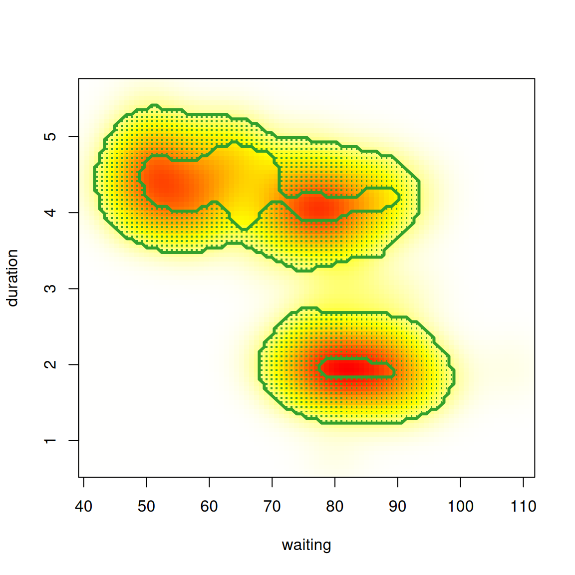plot(fs, addKDE=FALSE, addSignifCurvRegion=TRUE)

plot(fs, addSignifCurvData=TRUE, curvCol="cyan")