Kernel density estimate

Kernel density estimate for 1- to 6-dimensional data.

Usage

kde(x, H, h, gridsize, gridtype, xmin, xmax, supp=3.7, eval.points, binned, 
    bgridsize, positive=FALSE, adj.positive, w, compute.cont=TRUE, 
    approx.cont=TRUE, unit.interval=FALSE, density=FALSE, verbose=FALSE)

# S3 method for class 'kde'
predict(object, ..., x, zero.flag=TRUE)

Arguments

x: matrix of data values
H,h: bandwidth matrix/scalar bandwidth. If these are missing, Hpi or hpi is called by default.
gridsize: vector of number of grid points
gridtype: not yet implemented
xmin,xmax: vector of minimum/maximum values for grid
supp: effective support for standard normal
eval.points: vector or matrix of points at which estimate is evaluated
binned: flag for binned estimation.
bgridsize: vector of binning grid sizes
positive: flag if data are positive (1-d, 2-d). Default is FALSE.
adj.positive: adjustment applied to positive 1-d data
w: vector of weights. Default is a vector of all ones.
compute.cont: flag for computing 1% to 99% probability contour levels. Default is TRUE.
approx.cont: flag for computing approximate probability contour levels. Default is TRUE.
unit.interval: flag for computing log transformation KDE on 1-d data bounded on unit interval [0,1]. Default is FALSE.
density: flag if density estimate values are forced to be non-negative function. Default is FALSE.
verbose: flag to print out progress information. Default is FALSE.
object: object of class kde
zero.flag: deprecated (retained for backwards compatibilty)
...: other parameters

Value

A kernel density estimate is an object of class kde which is a list with fields:

x: data points - same as input
eval.points: vector or list of points at which the estimate is evaluated
estimate: density estimate at eval.points
h: scalar bandwidth (1-d only)
H: bandwidth matrix
gridtype: "linear"
gridded: flag for estimation on a grid
binned: flag for binned estimation
names: variable names
w: vector of weights
cont: vector of probability contour levels

Details

For d=1, if h is missing, the default bandwidth is hpi. For d>1, if H is missing, the default is Hpi.

For d=1, if positive=TRUE then x is transformed to log(x+adj.positive) where the default adj.positive is the minimum of x. This is known as a log transformation density estimate. If unit.interval=TRUE then x is transformed to qnorm(x). See kde.boundary for boundary kernel density estimates, as these tend to be more robust than transformation density estimates.

For d=1, 2, 3, and if eval.points is not specified, then the density estimate is computed over a grid defined by gridsize (if binned=FALSE) or by bgridsize (if binned=TRUE). This form is suitable for visualisation in conjunction with the plot method.

For d=4, 5, 6, and if eval.points is not specified, then the density estimate is computed over a grid defined by gridsize.

If eval.points is specified, as a vector (d=1) or as a matrix (d=2, 3, 4), then the density estimate is computed at eval.points. This form is suitable for numerical summaries (e.g. maximum likelihood), and is not compatible with the plot method. Despite that the density estimate is returned only at eval.points, by default, a binned gridded estimate is calculated first and then the density estimate at eval.points is computed using the predict method. If this default intermediate binned grid estimate is not required, then set binned=FALSE to compute directly the exact density estimate at eval.points.

Binned kernel estimation is an approximation to the exact kernel estimation and is available for d=1, 2, 3, 4. This makes kernel estimators feasible for large samples. The default value of the binning flag binned is n>1 (d=1), n>500 (d=2), n>1000 (d>=3). Some times binned estimation leads to negative density values: if non-negative values are required, then set density=TRUE.

The default bgridsize,gridsize are d=1: 401; d=2: rep(151, 2); d=3: rep(51, 3); d=4: rep(21, 4).

The effective support for a normal kernel is where all values outside [-supp,supp]^d are zero.

The default xmin is min(x)-Hmax*supp and xmax is max(x)+Hmax*supp where Hmax is the maximum of the diagonal elements of H. The grid produced is the outer product of c(xmin[1], xmax[1]), ..., c(xmin[d], xmax[d]). For ks \(\geq\) 1.14.0, when binned=TRUE and xmin,xmax are not missing, the data values x are clipped to the estimation grid delimited by xmin,xmax to prevent potential memory leaks.

Examples

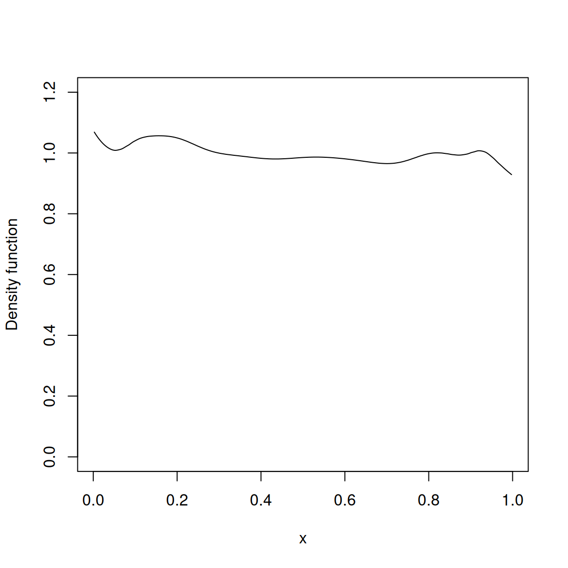
## unit interval data 
set.seed(8192)             
fhat <- kde(runif(10000,0,1), unit.interval=TRUE)
plot(fhat, ylim=c(0,1.2))


## positive data 
data(worldbank)
wb <- as.matrix(na.omit(worldbank[,2:3]))
wb[,2] <- wb[,2]/1000
fhat <- kde(x=wb)
fhat.trans <- kde(x=wb, adj.positive=c(0,0), positive=TRUE)
plot(fhat, col=1, xlim=c(0,20), ylim=c(0,80))
plot(fhat.trans, add=TRUE, col=2)
rect(0,0,100,100, lty=2)


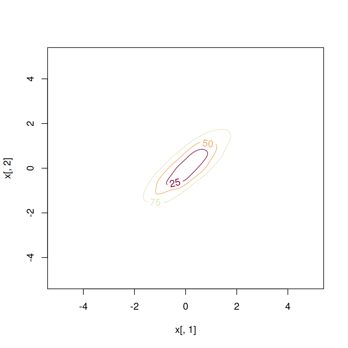
## large data on non-default grid
## 151 x 151 grid = [-5,-4.933,..,5] x [-5,-4.933,..,5]
set.seed(8192)
x <- rmvnorm.mixt(10000, mus=c(0,0), Sigmas=invvech(c(1,0.8,1)))
fhat <- kde(x=x, compute.cont=TRUE, xmin=c(-5,-5), xmax=c(5,5), bgridsize=c(151,151))
plot(fhat)


## See other examples in ? plot.kde