Plot for 1- to 3-dimensional normal and t-mixture density functions

Plot for 1- to 3-dimensional normal and t-mixture density functions.

Usage

plotmixt(mus, sigmas, Sigmas, props, dfs, dist="normal", draw=TRUE,
   deriv.order=0, which.deriv.ind=1, binned=TRUE, ...)

Arguments

mus

(stacked) matrix of mean vectors

sigmas

vector of standard deviations (1-d)

Sigmas

(stacked) matrix of variance matrices (2-d, 3-d)

props

vector of mixing proportions

dfs

vector of degrees of freedom

dist

"normal" - normal mixture, "t" - t-mixture

draw

flag to draw plot. Default is TRUE.

deriv.order

derivative order

which.deriv.ind

index of which partial derivative to plot

binned

flag for binned estimation of contour levels. Default is TRUE.

...

other graphics parameters, see plot.kde

Value

If draw=TRUE, the 1-d, 2-d plot is sent to graphics window, 3-d plot to graphics/RGL window. If draw=FALSE, then a kdde-like object is returned.

Examples

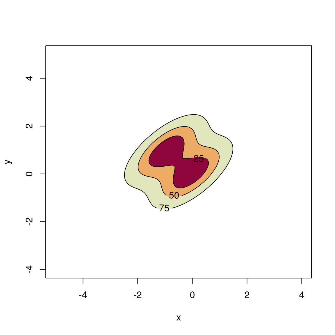
## bivariate 
mus <- rbind(c(0,0), c(-1,1))
Sigma <- matrix(c(1, 0.7, 0.7, 1), nr=2, nc=2) 
Sigmas <- rbind(Sigma, Sigma)
props <- c(1/2, 1/2)
plotmixt(mus=mus, Sigmas=Sigmas, props=props, display="filled.contour", lwd=1)


## trivariate 
mus <- rbind(c(0,0,0), c(-1,0.5,1.5))
Sigma <- matrix(c(1, 0.7, 0.7, 0.7, 1, 0.7, 0.7, 0.7, 1), nr=3, nc=3) 
Sigmas <- rbind(Sigma, Sigma)
props <- c(1/2, 1/2)
plotmixt(mus=mus, Sigmas=Sigmas, props=props, dfs=c(11,8), dist="t")