PRIM plot for multivariate data

PRIM plot for multivariate data.

Usage

# S3 method for class 'prim'
plot(x, splom=TRUE,  ...)

Arguments

x

object of class prim

splom

flag for plotting 3-d data as scatter plot matrix. Default is TRUE.

...

other graphics parameters

Value

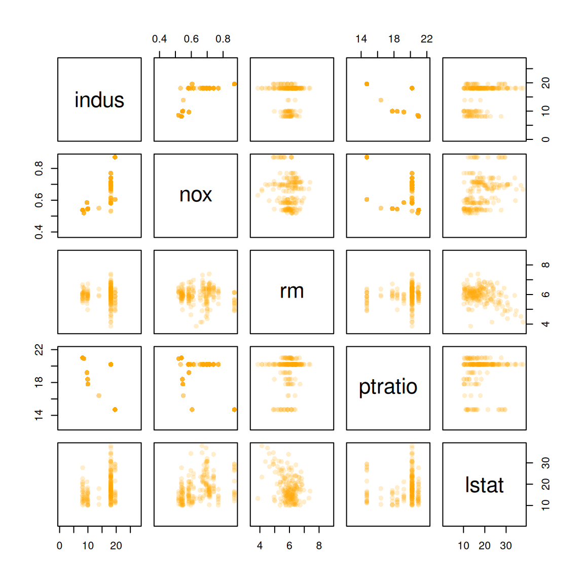
Plot of 2-dim PRIM is a set of nested rectangles. Plot of 3-dim PRIM is a scatter point cloud. Plot of d-dim PRIM is a scatter plot matrix. The scatter plots indicate which points belong to which box.

Details

The function headers are

  ## bivariate
  x, col, xlim, ylim, xlab, ylab, add=FALSE, add.legend=FALSE, cex.legend=1,
  pos.legend, lwd=1, border, col.vec=c("blue", "orange"), alpha=1, ...)

  ## trivariate
  plot(x, xlim, ylim, zlim, xlab, ylab, zlab, col.vec=c("blue","orange"),
  alpha=1, theta=30, phi=40, d=4, ...)

  ## d-variate
  plot(x, xmin, xmax, xlab, ylab, x.pt, m, col.vec=c("blue","orange"),
  alpha=1, ...)

The arguments are

add.legend

flag for adding legend (2-d plot)

pos.legend

(x,y) co-ordinates for legend (2-d plot)

cex.legend

cex graphics parameter for legend (2-d plot)

col.vec

vector of plotting colours, one for each box

xlab,ylab,zlab,xlim,ylim,zlim,add,lwd,alpha,phi,theta,d

usual graphics parameters

xmin,xmax

vector of minimum and maximum axis plotting values for scatter plot matrix

x.pt

data set to plot (other than x)

See also

prim.box, predict.prim

Examples

## see ?prim.box for bivariate example
## trivariate example
data(quasiflow)
qf <- quasiflow[1:1000,1:3]
qf.label <- quasiflow[1:1000,4]
thr <- c(0.25, -0.3)
qf.prim <- prim.box(x=qf, y=qf.label, threshold=thr, threshold.type=0)
plot(qf.prim, splom=FALSE, colkey=FALSE, alpha=0.5, pch=16)


## high-dimensional example
data(Boston, package="MASS")
x <- Boston[,c(3,5:6,11,13)]
y <- Boston[,1]
boston.prim <- prim.box(x=x, y=y, threshold.type=1)
plot(boston.prim, x.pt=x, alpha=0.2, pch=16)