 |
Hello. This talk is titled `Efficient day-to-day simulation of traffic
systems with applications to the effects of pre-trip information.' My name is Tarn Duong and this work was done with Dr Martin Hazelton at the University of Western Australia at the beginning of this year.
We are interested in modelling traffic systems. Early traffic systems models were chosen mostly because of their simple properties and were able to give exact, closed form solutions. With the advent of easily available fast computing power, many statistical techniques once considered to be computationally infeasible are now available. With these new techniques, we can now implement more realistic traffic systems models. However even for moderately sized networks, the computation time can still very large and further improvements need to be made so that the implementation is truly feasible. These ideas will be discussed in this talk. |
 |
First we will discuss the basic features of traffic systems models i.e. what features they should have in order to exhibit realistic behaviour.
The next section is about Markov assignment models which are a statistical tool for implementing traffic systems models. After that is on how to efficiently simulate these Markov models.
Finally we have an application of the software MARTS (Markov Assignment for Road Traffic Systems) to the effects of pre-trip information. |
 |
The level of the detail of the model is our first consideration.
In the models we will consider, travellers make informed decisions for today based on previous days's information so we have detailed day-to-day traveller learning. However there is no within-day traveller learning as once traveller has decided on a route, it is not changed according to changing conditions on that day. We note that here highly-detailed microscopic models (which allow within-day traveller learning) fit the data well as they fit a large number of parameters. However because of this potential for over-parametrisation, they have poor predictive qualities. Since we are mostly concerned with the moderate to long term behaviour of traffic systems, we use mesoscopic models. |
 |
Our second consideration is the type of route choice. Each route in the network has a measured disutility - this can be viewed as a cost that affects all travellers on the route equally.
Since each traveller has imperfect knowledge of the road network and hence the measured disutilities then each traveller has a perceived disutility which is the measured disutility plus a perceptual random error. This means that each traveller has a different perceived disutility for each route. The basic assumption that we use is that the traveller will then choose the route with the smallest perceived disutility. For probit route choice, each link (keeping in mind that a route is a sequence of links) has independent Normally distributed perceptual random errors. In this set-up, the exact route choice probabilities are mathematically intractable and so we need to estimate them by simulating Markov assignment models. |
 |
Markov assignment models are a statistical tool for implementing the traffic models of our choice namely mesoscopic day-to-day probit models. The basic
idea underlying Markov assignment is that a traveler's current perceived disutility is based on the previous disutilities.
A simple example is given on the slide. Suppose that only the previous two days affect today. Then in the example, a traveller gives most weight to what happened yesterday (i.e. 80 %) and only 20% weight to what happened on the day before yesterday. |
 |
As mentioned earlier, route choice probabilities for the probit model are impossible to compute exactly so we need to use simulation. The simulation algorithm that we use is
For each day and each traveller
As you can see, this is extremely computationally intensive as there can be thousands of travellers on a network with hundreds of links, all occurring over hundreds of days. |
 |
So we need to think of how to conduct these simulations efficiently. We have implemented several improvements. The first two (selective and implicit assignment) are theoretical improvements in the sense that they are independent of the actual implementation e.g. programming language or hardware. The third one however is concerned with the actual implementation and in particular, with efficient coding. |
 |
Selective assignment divides travellers into two classes: habitual and selective. Habitual travellers always select today's route to be exactly the same as the route that they took yesterday. In contrast, selective travellers consider all their perceived disutilities on their routes and choose the one that has the smallest perceived disutility. When this occurs this is known as explicit assignment.
If we run simulations with a high proportion of habitual travellers, we replicate observed traveller behaviour as it is usually the case that many travellers choose the same route everyday, despite changing conditions. If we run simulations with a high proportion of selective travellers then the network flows oscillate in an unrealistic manner. So by replicating realistic behaviour it is extremely fortunate that we also reduce the running time of our simulations. |
 |
Using implicit assignment also leads to less computation: from the explicitly assigned routes, we can then estimate the route choice probabilities. These will be just the estimated proportion of travellers taking each route. We then use these estimated route choice probabilities to randomly assign routes to the remaining travellers. This is known as implicit assignment. Because we don't need to simulate random perceptual errors and in particular find the actual minimum route, we require much less computation.
An example of implicit assignment is given on the slide. Suppose we have 500 travellers for a particular OD pair. We can assign routes to the first 200 travellers explicitly. From these 200 routes, we can then estimate the route choice probabilities which we then use to randomly assign routes according to a multinomial model with these estimated route choice probabilities to the remaining 300 travellers. |
 |
We now move onto efficient coding. The main programming language that we use is Splus and its clone R. These are state-of-the-art statistical analysis software packages. They are easy to program but are slow. On the other hand C is fast but less easy to program, especially for Markov assignment models. Since it is explicitly finding the shortest path that requires the most computing resources, the solution we arrived at is to code the shortest path finder in C and to dynamically load into Splus/ R. This way we preserve the ease of programming and reduce the computing time. |
 |
(Pause)
We now look at an application of the software to the effects of pre-trip information. The road network that we use is from the UK city of Leicester, in central England. Throughout the simulations, we examine how travellers react to the quality of the pre-trip information. This is controlled by the variance of the perceptual random error. (Show slide.) Here is a diagram of the network. London Road is a major arterial road that runs south-east to north-west, from node 5 to node 1. There are 14 nodes and 18 links. The main origin and destination nodes are nodes 1, 5, 6, 12, 13 and 14 (which are in red) with approximately 3800 travellers on this network, during a 1 hour period. |
 |
The full range of 6 scenarios is described in the paper that accompanies this talk. For brevity we will look at only 2 of these: scenario C where there is poor pre-trip information (20% variance) and scenario D where there is good pre-trip information (1% variance) We want to examine the moderate term behaviour of the travellers under these scenarios so they are simulated for 100 iterations. |
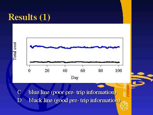 |
The results from this simulation are presented here. This is an actual plot from the software. On the horizontal axis is the iteration or day number. On the vertical axis is the total cost on the network. This is the sum of the actual costs for all travellers. Scenario C (the blue line) has a uniformly higher total cost than scenario D (black line). This is expected since the quality of pre-trip information is much better in scenario D.
|
 |
The software is capable of simulating more complicated situations. We extend the simulations by introducing road works in the link (2,3) which is in the middle of London Road after 100 days. These road works will halve the capacity n the left-right direction. The scenarios are then iterated for another 100 days. |
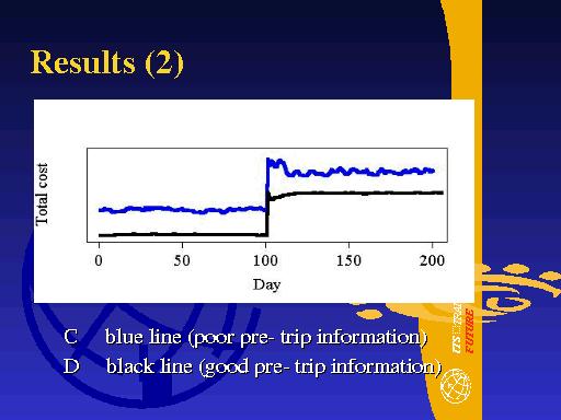 |
The results here show that there are breaks in the time series. For the first 100 days, we have the same situation as before. After the road works are introduced at day 100, both scenarios experience a marked increase in the total cost on the network. This again is expected as we have reduced the capacity of the major arterial route. Since there is congestion on London Road, the disutility of travelling on this route will increase markedly and this contributes to the increase of the total cost on the network.
Another important feature in these time series is that scenario D settles down to its new equilibrium faster than scenario C. Again this is because travellers under scenario D have better pre-trip information and so adjust faster to the changed road conditions.
|
 |
(Pause)
(Read slide.)
Thank you. |
These notes are part of a seminar given by the author on 3 Sept 2001 as part of the 8th World Congress on Intelligent Transporst Systems, Sydney, Australia. Please feel free to contact the author at tarn(at)duong(at)gmail(dot)com if you have any questions.