Kernel density estimate for bounded data

Kernel density estimate for bounded 1- to 3-dimensional data.

Usage

kde.boundary(x, H, h, gridsize, gridtype, xmin, xmax, supp=3.7, eval.points, 
   binned=FALSE, bgridsize, w, compute.cont=TRUE, approx.cont=TRUE,
   boundary.supp, boundary.kernel="beta", verbose=FALSE)

Arguments

x

matrix of data values

H,h

bandwidth matrix/scalar bandwidth. If these are missing, Hpi or hpi is called by default.

gridsize

vector of number of grid points

gridtype

not yet implemented

xmin,xmax

vector of minimum/maximum values for grid

supp

effective support for standard normal

eval.points

vector or matrix of points at which estimate is evaluated

binned

flag for binned estimation.

bgridsize

vector of binning grid sizes

w

vector of weights. Default is a vector of all ones.

compute.cont

flag for computing 1% to 99% probability contour levels. Default is TRUE.

approx.cont

flag for computing approximate probability contour levels. Default is TRUE.

boundary.supp

effective support for boundary region

boundary.kernel

"beta" = beta boundary kernel, "linear" = linear boundary kernel

verbose

flag to print out progress information. Default is FALSE.

Value

A kernel density estimate for bounded data is an object of class kde.

Details

There are two forms of density estimates which are suitable for bounded data, based on the modifying the kernel function. For boundary.kernel="beta", the 2nd form of the Beta boundary kernel of Chen (1999) is employed. It is suited for rectangular data boundaries.

For boundary.kernel="linear", the linear boundary kernel of Hazelton & Marshall (2009) is employed. It is suited for arbitrarily shaped data boundaries, though it is currently only implemented for rectangular boundaries.

References

Chen, S. X. (1999) Beta kernel estimators for density functions. Computational Statistics and Data Analysis, 31, 131–145.

Hazelton, M. L. & Marshall, J. C. (2009) Linear boundary kernels for bivariate density estimation. Statistics and Probability Letters 79, 999–1003.

See also

kde

Examples

data(worldbank)
wb <- as.matrix(na.omit(worldbank[,c("internet", "ag.value")]))
fhat <- kde(x=wb)
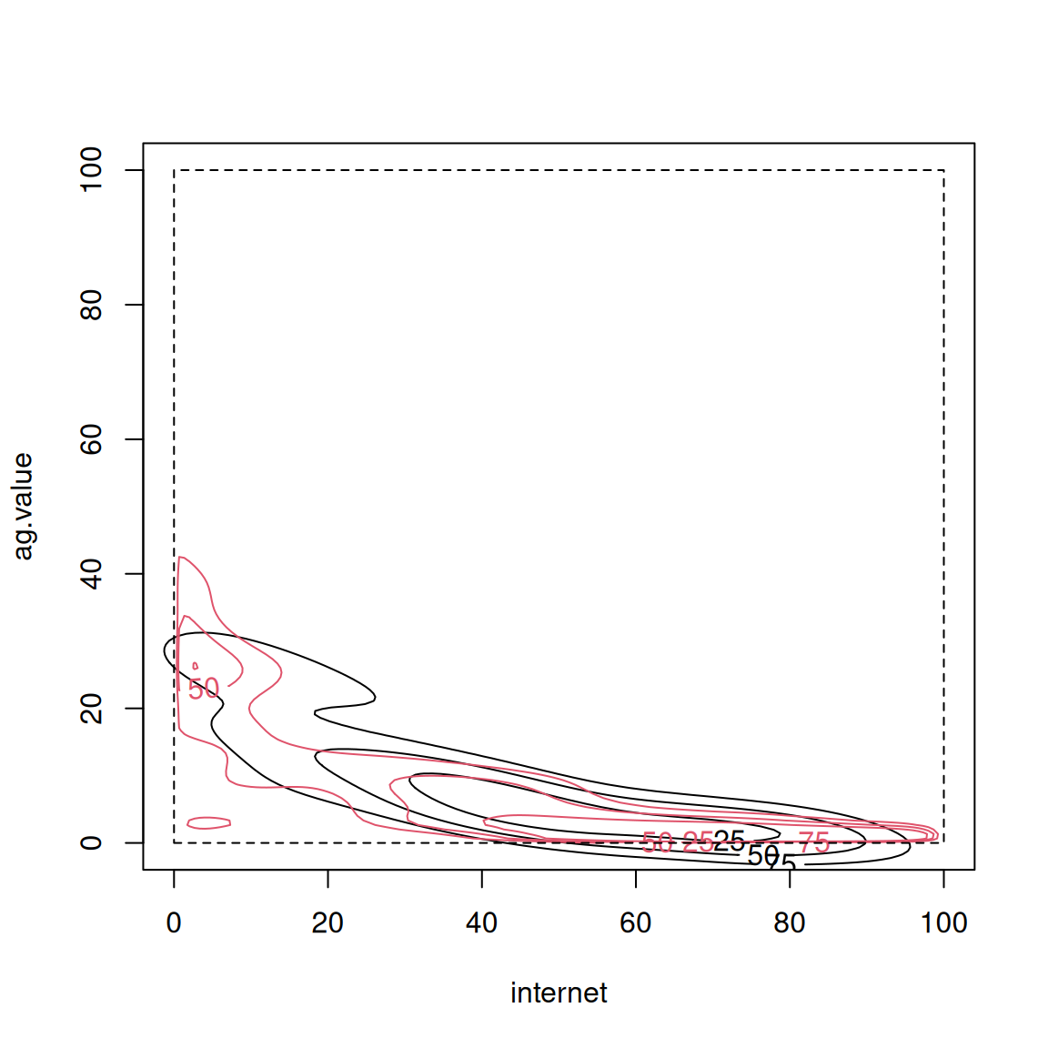
fhat.beta <- kde.boundary(x=wb, xmin=c(0,0), xmax=c(100,100), boundary.kernel="beta")  
plot(fhat, col=1, xlim=c(0,100), ylim=c(0,100))
plot(fhat.beta, add=TRUE, col=2)
rect(0,0,100,100, lty=2)


fhat.LB <- kde.boundary(x=wb, xmin=c(0,0), xmax=c(100,100), boundary.kernel="linear")
plot(fhat, col=1, xlim=c(0,100), ylim=c(0,100))
plot(fhat.LB, add=TRUE, col=3)
rect(0,0,100,100, lty=2)