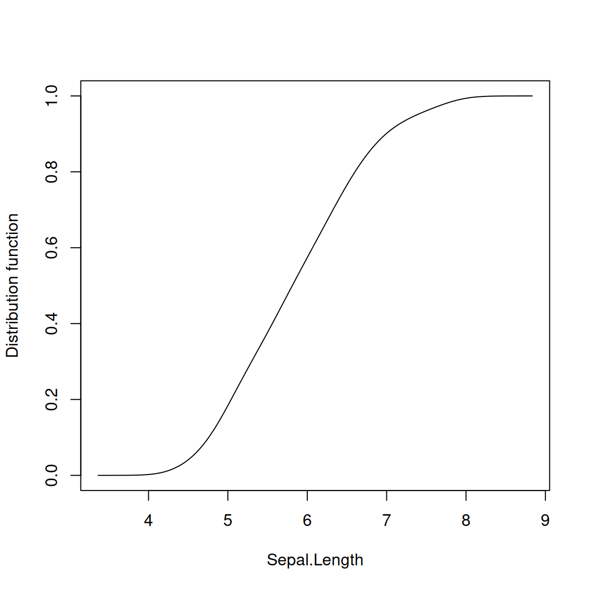
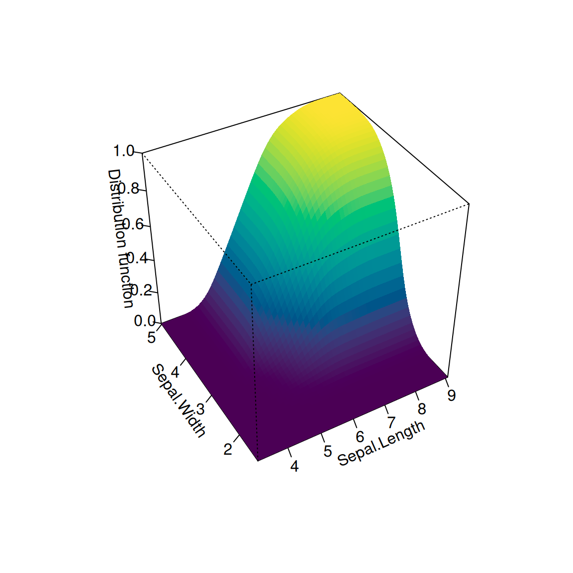
Plot for kernel cumulative distribution estimate

Plot for kernel cumulative distribution estimate 1- to 3-dimensional data.

Usage

# S3 method for class 'kcde'
plot(x, ...)

Arguments

x: object of class kcde (output from kcde)
...: other graphics parameters used in plot.kde

Value

Plots for 1-d and 2-d are sent to graphics window. Plot for 3-d is sent to graphics/RGL window.

Details

For kcde objects, the function headers for the different dimensional data are


  ## univariate
  plot(Fhat, xlab, ylab="Distribution function", add=FALSE, drawpoints=FALSE,
       col.pt=4, jitter=FALSE, alpha=1, ...)

  ## bivariate
  plot(Fhat, display="persp", cont=seq(10,90, by=10), abs.cont, xlab, ylab,
       zlab="Distribution function", cex=1, pch=1, add=FALSE, drawpoints=FALSE,
       drawlabels=TRUE, theta=-30, phi=40, d=4, col.pt=4, col, col.fun, alpha=1,
       lwd=1, border=NA, thin=3, lwd.fc=5, ...)

  ## trivariate
  plot(Fhat, display="plot3D", cont=c(25,50,75), colors, col, alphavec,
       size=3, cex=1, pch=1, theta=-30, phi=40, d=4, ticktype="detailed",
       bty="f", col.pt=4, add=FALSE, xlab, ylab, zlab, drawpoints=FALSE,
       alpha, box=TRUE, axes=TRUE, ...)

Examples

data(iris)
Fhat <- kcde(x=iris[,1])
plot(Fhat, xlab="Sepal.Length")

Fhat <- kcde(x=iris[,1:2])
plot(Fhat)

Fhat <- kcde(x=iris[,1:3])
plot(Fhat, alpha=0.3)