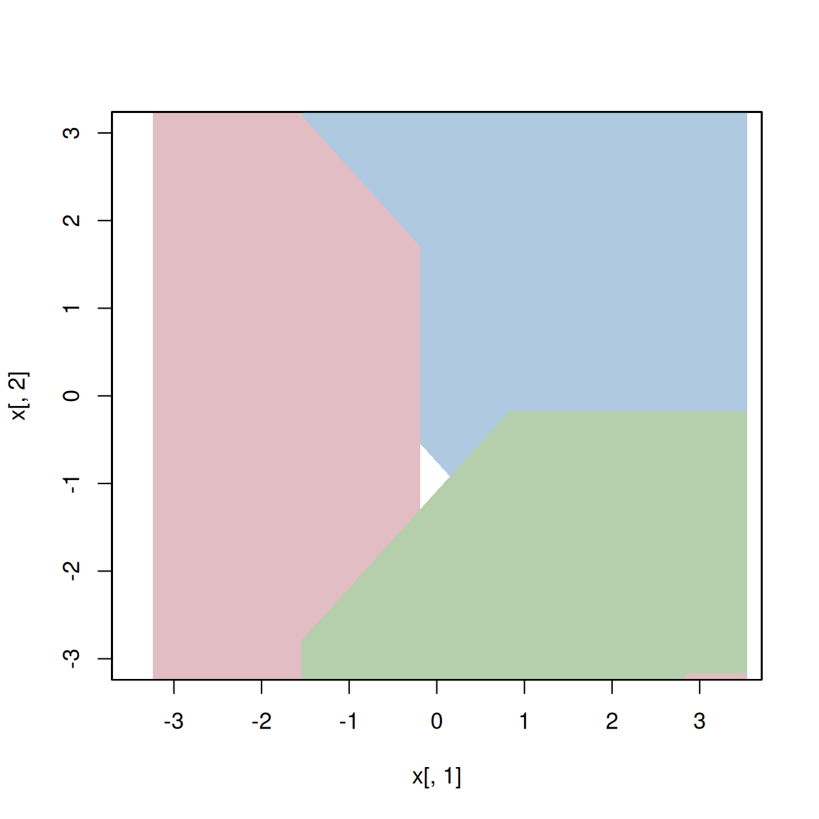
Partition plot for kernel density clustering

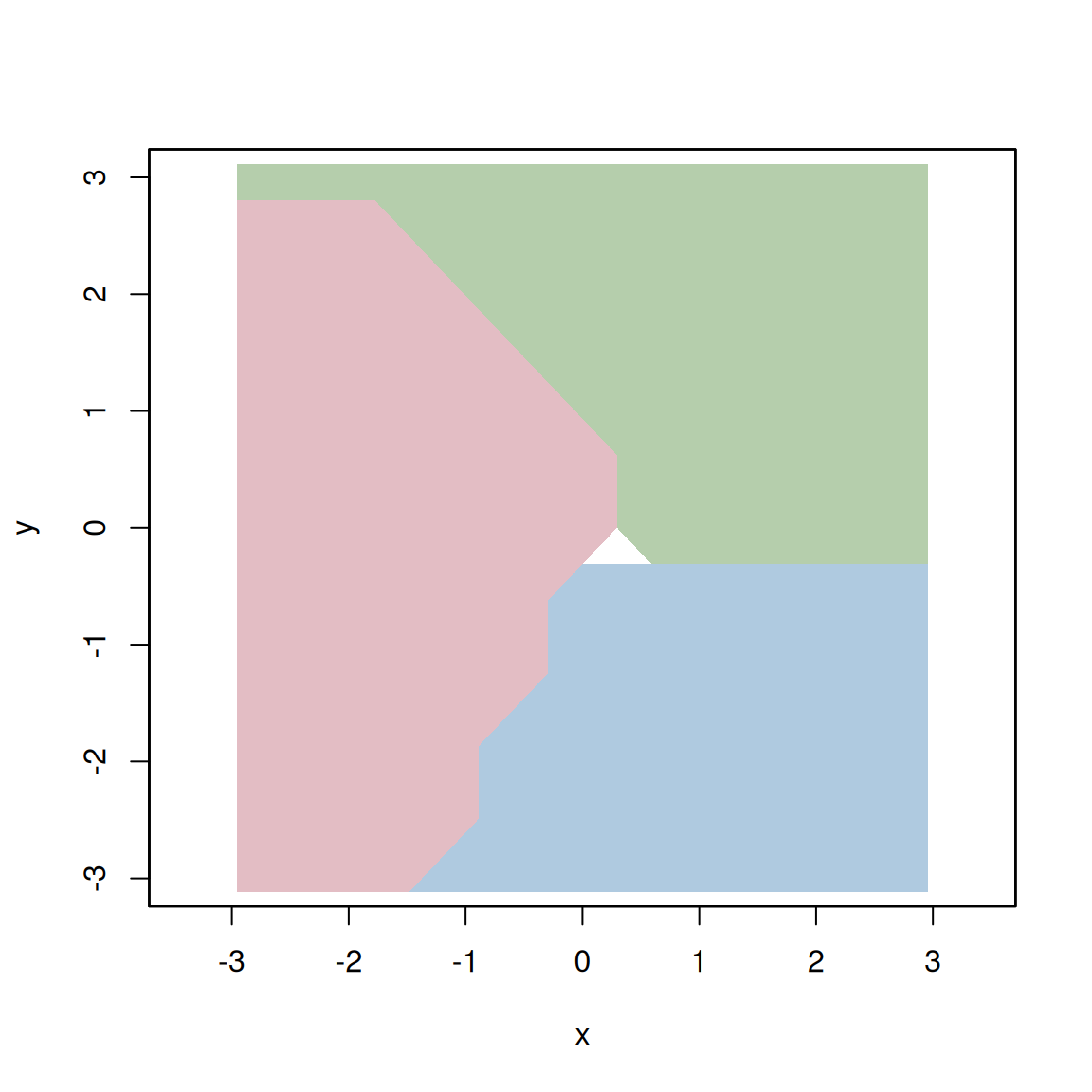
Plot of partition for kernel density clustering for 2-dimensional data.

Usage

mvnorm.mixt.part(mus, Sigmas, props=1, xmin, xmax, gridsize, max.iter=100,
   verbose=FALSE)
kms.part(x, H, xmin, xmax, gridsize, verbose=FALSE, ...)

# S3 method for class 'kde.part'
plot(x, display="filled.contour", col, col.fun, alpha=1, add=FALSE, ...)

Arguments

mus: (stacked) matrix of mean vectors
Sigmas: (stacked) matrix of variance matrices
props: vector of mixing proportions
xmin,xmax: vector of minimum/maximum values for grid
gridsize: vector of number of grid points
max.iter: maximum number of iterations
verbose: flag to print out progress information. Default is FALSE.
x: matrix of data values or an object of class kde.part
H: bandwidth matrix. If missing, Hpi(x,deriv,order=1) is called by default.
display: type of display, "filled.contour" for filled contour plot
col,col.fun: vector of plotting colours or colour function
alpha: colour transparency. Default is 1.
add: flag to add to current plot. Default is FALSE.
...: other parameters

Value

A kernel partition is an object of class kde.part which is a list with fields:

x: data points - same as input
eval.points: vector or list of points at which the estimate is evaluated
estimate: density estimate at eval.points
H: bandwidth matrix
gridtype: "linear"
gridded: flag for estimation on a grid
binned: flag for binned estimation
names: variable names
w: vector of weights
cont: vector of probability contour levels
end.points: matrix of final iterates starting from x
label: vector of cluster labels
mode: matrix of cluster modes
nclust: number of clusters
nclust.table: frequency table of cluster labels
tol.iter,tol.clust,min.clust.size: tuning parameter values - same as input

Plot is sent to graphics window.

Details

For 2-d data, kms.part and mvnorm.mixt.part produce a kde.part object whose values are the class labels, rather than probability density values.

Examples

## normal mixture partition
mus <- rbind(c(-1,0), c(1, 2/sqrt(3)), c(1,-2/sqrt(3)))
Sigmas <- 1/25*rbind(invvech(c(9, 63/10, 49/4)), invvech(c(9,0,49/4)), invvech(c(9,0,49/4)))
props <- c(3,3,1)/7
gridsize <- c(11,11) ## small gridsize illustrative purposes only 
nmixt.part <- mvnorm.mixt.part(mus=mus, Sigmas=Sigmas, props=props, gridsize=gridsize)
plot(nmixt.part, asp=1, xlim=c(-3,3), ylim=c(-3,3), alpha=0.5)


## kernel mean shift partition
set.seed(81928192)
x <- rmvnorm.mixt(n=10000, mus=mus, Sigmas=Sigmas, props=props)
msize <- round(prod(gridsize)*0.1)
kms.nmixt.part <- kms.part(x=x, min.clust.size=msize, gridsize=gridsize)
plot(kms.nmixt.part, asp=1, xlim=c(-3,3), ylim=c(-3,3), alpha=0.5)