Contour functions for tidy and geospatial kernel estimates

Contour functions for tidy and geospatial kernel estimates.

Usage

# S3 method for class 'tidy_ks'
contourLevels(x, ..., cont=c(25,50,75))
# S3 method for class 'sf_ks'
contourLevels(x, ..., cont=c(25,50,75))
contour_breaks(data, cont=c(25,50,75), n=3, group=FALSE, type="density")
st_get_contour(x, cont=c(25,50,75), breaks, disjoint=TRUE, digits)
add_contour_breaks(x, breaks, digits, ...)

Arguments

x,data: tidy kernel estimate (output from tidy_k*) or geospatial kernel estimate (output from st_k*)
cont: vector of contour levels. Default is c(25,50,75). Used only for level="density", "quantile".
n: number of contour levels. Default is 3. Used only for level="length", "natural".
type: type of contour levels: one of "density", "length", "quantile", "natural". Default is "density".
group: flag to compute contour levels per group. Default is FALSE.
breaks: tibble or vector of contour levels (e.g. output from contour_breaks)
disjoint: flag to compute disjoint contours. Default is TRUE.
digits: number of significant digits in output labels. If missing, default is 4.
...: parameters to contour_breaks (only for add_contour_breaks)

Value

–The output from contour_breaks is a tibble of the values of the contour breaks. If group=FALSE then a single set of contour breaks is returned. If group=TRUE then a set of contour breaks for each group is returned.

–The output from st_get_contour is an sf object of the contours as multipolygons, with added attributes

estimate: density value or factor with digits s.f.
contlabel: factor of contour probability level
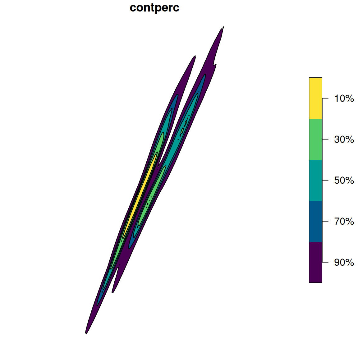
contperc: factor of contour probability level with added %
contregion: factor of contour probability level with added \(\leq\) or \(\geq\)

These are used to render the contours in the base R base graphics, and via the aesthetics in ggplot.

Details

By default, the 5%, 10%, ..., 95% contours are computed for an st_k* output, though a plot of 19 of them would be too crowded. st_get_contour selects a subset of these, as specified by cont. If a contour level in cont does not already exist or if absolute contour levels are specified in breaks, then the corresponding contours are computed. If disjoint=TRUE (default) then the contours are computed as a set of disjoint multipolygons: this allows for plotting without overlapping transparent colours. If disjoint=FALSE then the contours are overlapping and so their colours alpha-mixed, but they strictly satisfy the probabilistic definition, e.g. a 25% contour region is the smallest region that contains 25% of the probability mass defined by the kernel estimate, see geom_contour_ks.

Since these default probability contours are relative contour levels, they are not suitable for producing a contour plot with fixed contour levels across all groups. It may require trial and error to obtain a single set of contour levels which is appropriate for all groups: one possible choice is provided by contour_breaks.

Examples

library(ggplot2)
#> Want to understand how all the pieces fit together? Read R for Data
#> Science: https://r4ds.hadley.nz/
theme_set(theme_bw())
data(crabs, package="MASS")
## tidy data 
crabs2 <- dplyr::select(crabs, FL, CW)
t1 <- tidy_kde(crabs2)
ggplot(t1, aes(x=FL, y=CW)) + geom_contour_filled_ks()


## add density contour region labels  
add_contour_breaks(t1, group=TRUE)
#> # A tibble: 22,801 × 7
#>       FL    CW estimate contregion ks        tks   label  
#>    <dbl> <dbl> <ord>    <fct>      <list>    <chr> <chr>  
#>  1  4.79  7.10 0        ≥ 0        <kde>     kde   Density
#>  2  4.93  7.10 0        ≥ 0        <int [1]> kde   Density
#>  3  5.06  7.10 0        ≥ 0        <int [1]> kde   Density
#>  4  5.20  7.10 0        ≥ 0        <int [1]> kde   Density
#>  5  5.34  7.10 0        ≥ 0        <int [1]> kde   Density
#>  6  5.48  7.10 0        ≥ 0        <int [1]> kde   Density
#>  7  5.62  7.10 0        ≥ 0        <int [1]> kde   Density
#>  8  5.75  7.10 0        ≥ 0        <int [1]> kde   Density
#>  9  5.89  7.10 0        ≥ 0        <int [1]> kde   Density
#> 10  6.03  7.10 0        ≥ 0        <int [1]> kde   Density
#> # ℹ 22,791 more rows

## geospatial data
crabs2s <- sf::st_as_sf(crabs2, coords=c("FL","CW"))
s1 <- st_kde(crabs2s)
s1_cont <- st_get_contour(s1, cont=seq(10,90, by=20))

## base R plot
vc <- function(.) colorspace::sequential_hcl(palette="viridis", n=.)
plot(s1_cont[,"contperc"], pal=vc)


## ggplot
ggplot() + scale_fill_viridis_d() + 
    geom_sf(data=s1_cont, aes(fill=contperc))