Tidy and geospatial kernel density derivative estimates
tidyst_kdde.RdTidy and geospatial versions of kernel density derivative estimates for 1- and 2-dimensional data.
Arguments
- data
data frame/tibble of data values
- deriv_order
derivative order. Default is 1.
- x
sf object with point geometry
- ...
other parameters in
ks::kddefunction
Value
–For tidy_kdde, the output is an object of class tidy_ks, which is a tibble with columns:
- x
evaluation points in x-axis (name is taken from 1st input variable in
data)- y
evaluation points in y-axis (2-d) (name is taken from 2nd input variable in
data)- estimate
kernel density derivative estimate values
- deriv_order
derivative order (same as input)
- deriv_ind
index of partial derivative
- ks
first row (within each
group) contains the untidy kernel estimate fromks::kde- tks
short object class label derived from the
ksobject class- label
long object class label
- group
grouping variable (if grouped input) (name is taken from grouping variable in
data)- deriv_group
additional derived grouping variable on partial derivative indices.
–For st_kdde, the output is an object of class st_ks, which is a list with fields:
- tidy_ks
tibble of simplified output (
deriv_ind,ks,tks,label,group,deriv_group) fromtidy_kdde- grid
sf object of grid of kernel density derivative estimate values, as polygons, with attributes
estimate,deriv_ind,group,deriv_groupcopied from thetidy_ksobject- sf
sf object of 5%, 10%, ..., 95% contour regions of the kernel density derivative estimate, as multipolygons, with attributes
estimate,contlabel,contperc,contregion,contlinederived from the contour level, andderiv_ind,group,deriv_groupcopied from thetidy_ksobject.
Details
The output from *_kdde have the same structure as the kernel density estimate from *_kde, except that estimate is the kernel density derivative values at the grid points, and the additional derived grouping variable deriv_group is the index of the partial derivative, e.g. "deriv (1,0)" and "deriv (0,1)" for a first order derivative for 2-d data. The output is a grouped tibble, grouped by the input grouping variable (if it exists) and by deriv_group.
For details of the computation of the kernel density derivative estimate and the bandwidth selector procedure, see ?ks::kdde.
In geom_contour_filled_ks and st_get_contour, the 100% contour
is set to the bounding box of the data, and it is plotted in a transparent (if data is not missing) or neutral colour (if data is missing). For geom_contour_filled_ks, it is difficult to avoid displaying the boundary of this bounding box , though for geom_sf, using aes(linetype=contline) achieves this.
See *_kde for details on the aesthetics based on contperc, contregion, estimate.
Examples
library(ggplot2)
data(crabs, package="MASS")
## 1-d density curvature estimate
crabs1 <- dplyr::select(crabs, FL)
t1 <- tidy_kdde(crabs1, deriv_order=2)
gt1 <- ggplot(t1, aes(x=FL))
gt1 + geom_line(colour=1)
 ## 2-d density gradient estimate
crabs2 <- dplyr::select(crabs, FL, CW)
t2 <- tidy_kdde(crabs2, deriv_order=1)
tb1 <- contour_breaks(t2, group=FALSE)
tb2 <- contour_breaks(t2, group=TRUE)
gt2 <- ggplot(t2, aes(x=FL, y=CW))
## overall set of contour breaks suitable for both derivatives
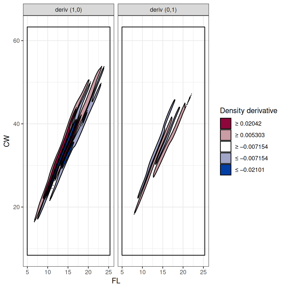
## filled contour regions with density derivative labels w/o breaks
## displays bounding box by default
gt2 + geom_contour_filled_ks(data=t2, aes(fill=after_stat(contregion)),
colour=1, breaks=tb1) + facet_wrap(~deriv_group)
## 2-d density gradient estimate
crabs2 <- dplyr::select(crabs, FL, CW)
t2 <- tidy_kdde(crabs2, deriv_order=1)
tb1 <- contour_breaks(t2, group=FALSE)
tb2 <- contour_breaks(t2, group=TRUE)
gt2 <- ggplot(t2, aes(x=FL, y=CW))
## overall set of contour breaks suitable for both derivatives
## filled contour regions with density derivative labels w/o breaks
## displays bounding box by default
gt2 + geom_contour_filled_ks(data=t2, aes(fill=after_stat(contregion)),
colour=1, breaks=tb1) + facet_wrap(~deriv_group)
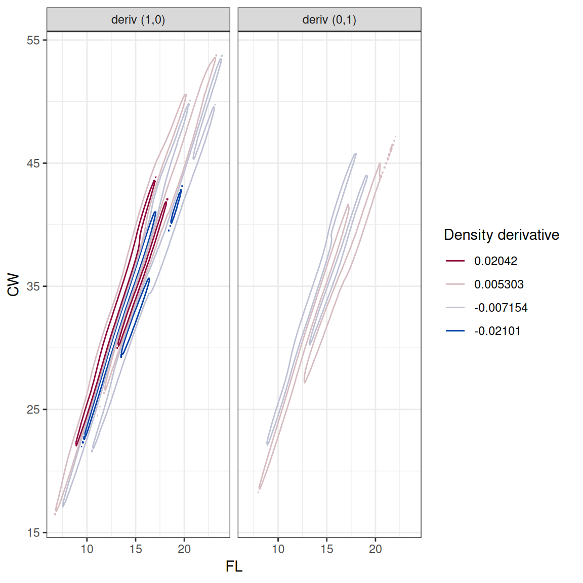
 ## contour lines with density derivative labels with breaks
gt2 + geom_contour_ks(data=t2, aes(group=deriv_group,
colour=after_stat(estimate)), breaks=tb1) + facet_wrap(~deriv_group)
## contour lines with density derivative labels with breaks
gt2 + geom_contour_ks(data=t2, aes(group=deriv_group,
colour=after_stat(estimate)), breaks=tb1) + facet_wrap(~deriv_group)
 ## second partial derivative f^(0,1) only
t22 <- dplyr::filter(t2, deriv_ind==2)
tb22 <- dplyr::filter(tb2, deriv_ind==2)
## filled contour regions with density derivative labels with breaks
## aes(linetype=after_stat(contline)) suppresses displaying bounding box
gt2 + geom_contour_filled_ks(data=t22, aes(fill=after_stat(contregion),
linetype=after_stat(contline)), colour=1, breaks=tb22)
## second partial derivative f^(0,1) only
t22 <- dplyr::filter(t2, deriv_ind==2)
tb22 <- dplyr::filter(tb2, deriv_ind==2)
## filled contour regions with density derivative labels with breaks
## aes(linetype=after_stat(contline)) suppresses displaying bounding box
gt2 + geom_contour_filled_ks(data=t22, aes(fill=after_stat(contregion),
linetype=after_stat(contline)), colour=1, breaks=tb22)
 ## contour lines with density derivative labels with breaks
gt2 + geom_contour_ks(data=t22, aes(colour=after_stat(estimate)),
breaks=tb22)
## contour lines with density derivative labels with breaks
gt2 + geom_contour_ks(data=t22, aes(colour=after_stat(estimate)),
breaks=tb22)
 ## geospatial density derivative estimate
data(wa)
data(grevilleasf)
hakeoides <- dplyr::filter(grevilleasf, species=="hakeoides")
s1 <- st_kdde(hakeoides, deriv_order=1)
## overall set of contour breaks suitable for both derivatives
sb1 <- contour_breaks(s1, group=FALSE)
s1_cont1 <- st_get_contour(s1, breaks=sb1)
## set of contour breaks per derivative
sb2 <- contour_breaks(s1, group=TRUE)
sb2 <- dplyr::filter(sb2, deriv_ind==2)
s1_cont2 <- st_get_contour(s1)
s1_cont2 <- dplyr::filter(s1_cont2, deriv_ind==2)
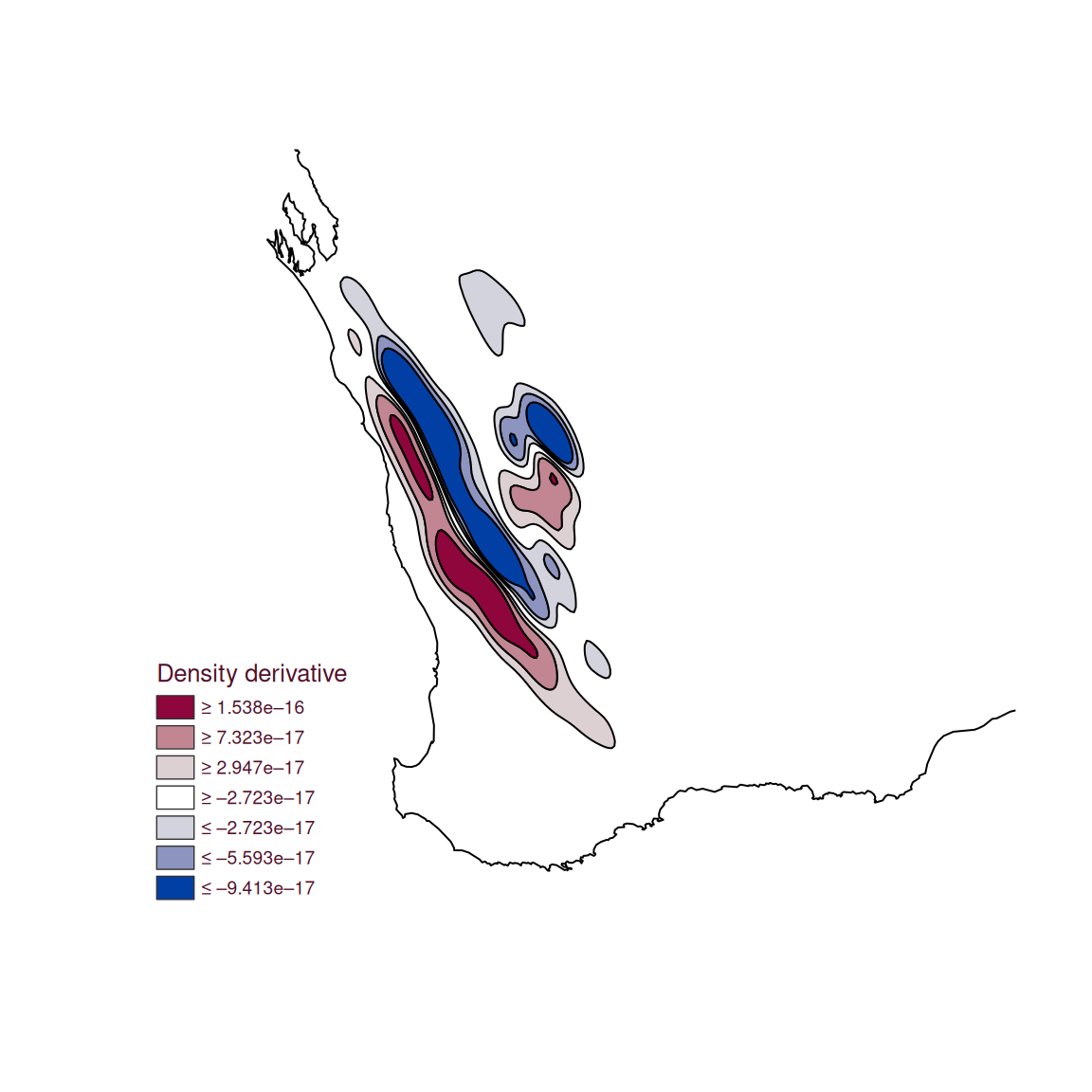
## base R plot
## filled contour regions with density derivative labels with breaks
xlim <- c(1.2e5, 1.1e6); ylim <- c(6.1e6, 7.2e6)
plot(wa, xlim=xlim, ylim=ylim)
plot(s1, add=TRUE, which_deriv_ind=2, breaks=sb2)
## geospatial density derivative estimate
data(wa)
data(grevilleasf)
hakeoides <- dplyr::filter(grevilleasf, species=="hakeoides")
s1 <- st_kdde(hakeoides, deriv_order=1)
## overall set of contour breaks suitable for both derivatives
sb1 <- contour_breaks(s1, group=FALSE)
s1_cont1 <- st_get_contour(s1, breaks=sb1)
## set of contour breaks per derivative
sb2 <- contour_breaks(s1, group=TRUE)
sb2 <- dplyr::filter(sb2, deriv_ind==2)
s1_cont2 <- st_get_contour(s1)
s1_cont2 <- dplyr::filter(s1_cont2, deriv_ind==2)
## base R plot
## filled contour regions with density derivative labels with breaks
xlim <- c(1.2e5, 1.1e6); ylim <- c(6.1e6, 7.2e6)
plot(wa, xlim=xlim, ylim=ylim)
plot(s1, add=TRUE, which_deriv_ind=2, breaks=sb2)
 ## geom_sf plot
glim <- coord_sf(xlim=xlim, ylim=ylim)
gs <- ggplot(s1) + geom_sf(data=wa, fill=NA) + theme_sf()
## filled contours with density derivative "percentage" labels w/o breaks
## aes(linetype=contline) suppresses displaying bounding box
gs + geom_sf(data=s1_cont2, aes(fill=contregion, linetype=contline),
colour=1) + scale_linetype_manual(values=c(0,1)) + glim
## geom_sf plot
glim <- coord_sf(xlim=xlim, ylim=ylim)
gs <- ggplot(s1) + geom_sf(data=wa, fill=NA) + theme_sf()
## filled contours with density derivative "percentage" labels w/o breaks
## aes(linetype=contline) suppresses displaying bounding box
gs + geom_sf(data=s1_cont2, aes(fill=contregion, linetype=contline),
colour=1) + scale_linetype_manual(values=c(0,1)) + glim
 ## facet wrapped geom_sf plot for each partial derivative
## filled contours with density derivative labels with breaks
gs + geom_sf(data=s1_cont1, aes(fill=contregion, linetype=contline)) +
scale_linetype_manual(values=c(0,1)) + glim + facet_wrap(~deriv_group)
## facet wrapped geom_sf plot for each partial derivative
## filled contours with density derivative labels with breaks
gs + geom_sf(data=s1_cont1, aes(fill=contregion, linetype=contline)) +
scale_linetype_manual(values=c(0,1)) + glim + facet_wrap(~deriv_group)
